Home  │ Audio Home Page

Copyright © 2013 by Wayne Stegall
Updated December 9, 2015.  See Document History at end for details.

Single-slope Safe-area Limiter

Introduction

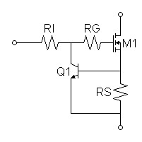
There are several transistor limiter circuits of which the singe-slope safe-area limiter is the most interesting.  All use the turn-on voltage (V_T) of a bipolar transistor to trigger the desired limit.  This V_T may not be the usual 0.7-1V of normal operation but rather a 0.60-0.65 required to barely turn the bipolar transistor on depending on how much current the input signal can supply to the collector of Q₁ under limit..

Current Limiter

The current limiter of figure 1 below measures current with the shunt resistor (R_S) whose value is chosen to turn on the bipolar transistor when the current limit is reached.  This circuit becomes a current source instead if the input to R_I is taken from an appropriate DC bias.

Figure 1:  Current Limiter

(1)

ILIMIT =

VT RS

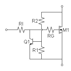
Voltage Limiter

The voltage limiter of figure 2 below uses a resistive voltage ladder to scale the desired voltage limit to the bipolar turn-on threshold..

Figure 2:  Voltage Limiter

(2)

VLIMIT =

R1 + R2 R1

× VT

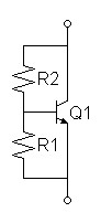
Because power supplies are typically constant voltage, transistors are chosen with voltage limits in excess of supply voltage and therefore usually do not need protection from overvoltage in isolation.  The voltage limiter is instead more often used for voltage biasing and appears most often in the circuit of figure 3, the amplified diode.

Figure 3:  Amplified diode

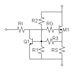
Single Slope Safe-area Limiter

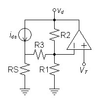
If the previous limiters were overly simple, the safe-area limiter of figure 4 becomes much more complex.  Here voltage and current signals are combined to limit the weighted sum of the two.  Under limiting conditions this circuit acts as a negative resistance.  This circuit becomes strictly a negative resistance instead if the input to R_I is taken from an appropriate DC bias.

Figure 4:  Safe-area Limiter

Graphical Analysis

It is useful at first for understanding to examine the graphical analysis of this circuit.  Begin a plot with specified load line and power limitations.

Figure 5:  Specified load-line and power limit boundaries

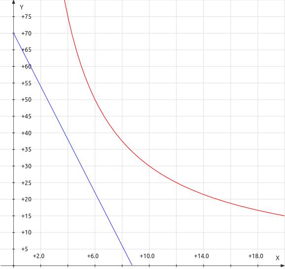Legend: — load line — power limit

Then plot a limit line between the load line and the curve representing the power dissipation limit.  In figure 6 below, a limit parallel with load line and touching the maximum power dissipation line is drawn.  Any limit in the range between the load line and power limit could be plotted, so figure 7 below shows a limit line more likely to cause limiting on signal peaks.

Figure 6:  Illustration of a parallel limit line positioned for maximum power

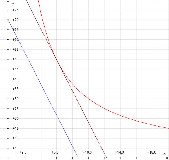Legend: — load line — power limit — limit line

Figure 7:  Illustration of a limit more likely to activate at peak signal

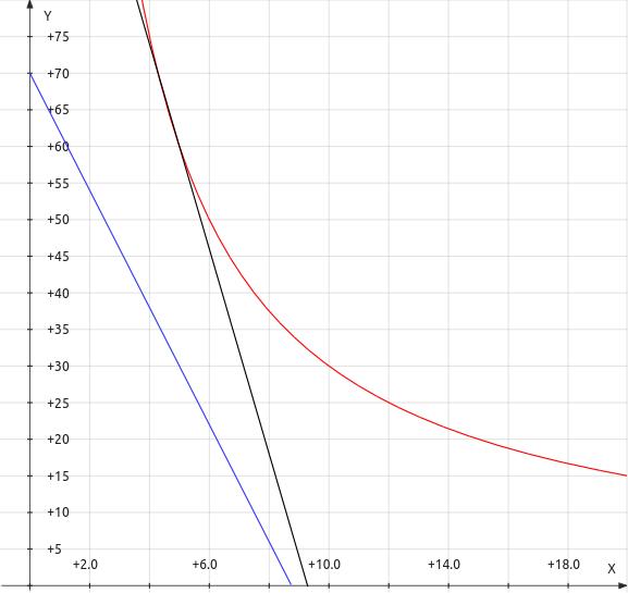Legend: — load line — power limit — limit line

Once a limit line is established, it can be defined by calculating two end-points

Mathematical Analysis

At this point it would be desirable to choose R₁ and calculate R₂ and R₃, however doing so would require solution of simultaneous non-linear equations.  It is therefore desirable to specify the limit line in more general terms before calculating R₂ and R₃ by numerical methods.

Therefore specify a general limit line equation

(3)	kvVDS + kiIDS = VT

At this point the desire to place the limit line tangent to a maximum power curve requires power calculations:

(4)

VDS =

VT - kiIDS kv

=

VT kv

–

ki kv

IDS

(5)

P = IDSVDS = IDS

VT kv

–

ki kv

IDS

(6)

P = –

ki kv

IDS2

+

VT kv

IDS

Now take the derivative of power to locate maximum power point

(7)

dP dIDS

= –

2ki kv

IDS

+

VT kv

= 0

Maximum power occurs where the slope of the power is zero

(8)

2ki kv

IDS

=

VT kv

(9)

IDS

=

VT 2ki

Now substitute the maximum power point back into the original power equation:

(10)

PMAX =

VT kv

VT 2ki

–

ki kv

VT 2ki

2

(11)

PMAX =

VT2 2kvki

–

kiVT2 4kvki2

=

VT2 2kvki

–

VT2 4kvki

(12)

PMAX =

VT2 4kvki

If ZLIM = -

ki kv

, then ki = |ZLIM|kv

Therefore

(13)

PMAX =

VT2 4|ZLIM|kv2

(14)

kv =

VT2 4|ZLIM|PMAX

At this point the general limit equation can be specified from the desired slope and maximum power limitation.

Component Calculations

Calculate k_v from the endpoint conditions:  V_DS = V_DS-MAX and I_DS = 0

Where k_vV_DS = V_T:

(15)

kv =

R1 || R3 (R1 || R3) + R2

Calculate k_i from the endpoint conditions:  V_DS = 0 and I_DS = I_DS-MAX

Where k_vV_DS = V_T:

(16)

ki =

R1 || R2 (R1 || R2) + R3

The general limit line from equation 3 now becomes:

(17)

R1 || R3 (R1 || R3) + R2

VD +

R1 || R2 (R1 || R2) + R3

IDS = VT

Although the value of R₂ is generally tied to the V_DS-MAX endpoint specified by k_v and R₃ to the I_DS-MAX endpoint specified by k_i, both resistances appear in both endpoint equations.  This entanglement requires numerical computation.  Now specify the calculations required.

Recursive equation for R₂

Solve equation 15 for R₂:

(18)

(R1 || R3) + R2 =

R1 || R3 kv

(19)

R2 =

R1 || R3 kv

– (R1 || R3)

Recursive equation for R₃

Solve equation 16 for R₃:

(20)

(R1 || R2) + R3 =

R1 || R2 ki

(21)

R3 =

R1 || R2 ki

– (R1 || R2)

The numerical calculation of R₂ and R₃ involves calculating equations 19 and 21 repeatedly until the results converge and do not change.

Figure 8:  C++ code for calculating safe-area limiter component values

/*     sal.cpp - prove the equations calculated to define     a single-slope safe area limiter. */ #include <iostream> #include <cmath> using namespace std; #define PAR(x,y) ((x)*(y)/((x)+(y))) /* If convergence is at least as good as binary, iterations equal to the number of bits in the mantissa of a double are sure to produce double accuracy */ #define ITER 52 int main(void) {     int i;     double zlim, pmax, kv, ki, vt;     double r1, r2, r3, rs, rtmp;     double vmax, imax;          // input values     zlim = 8.0;     pmax = 300.0;     r1 = 68.0;     rs = 0.1;     vt = 0.763;     // calculate limit line specifications     kv = sqrt((vt*vt)/(4.0*zlim*pmax));     ki = kv*zlim;     vmax = vt/kv;     imax = vt/ki;          // calculate component values     r2 = r1;     r3 = r1;     for(i=0;i<ITER;i++)     {         rtmp = PAR(r1,r3);         r2 = (rtmp/kv)-rtmp;         rtmp = PAR(r1,r2);         r3 = (rs*rtmp/ki)-rtmp;                          // watch results for convergence         cout << "R2 = " << r2 << ",\t" << "R3 = " << r3 << endl;     }     // print remaining results     cout << "Seed values:" << endl;     cout << "R1 = " << r1 << ",\t" << "RS = " << rs << endl;     cout << "VT = " << vt << ",\t" << "PMAX = " << pmax;     cout << ",\t" << "ZLIM = " << zlim << endl;     cout << "Endpoints: " << vmax << "V,\t" << imax << "A" << endl;     return 0; }

Figure 9:  Program output for parameters given

R2 = 4332.06,    R3 = 40.5156 R2 = 3234.86,    R3 = 40.3043 R2 = 3224.26,    R3 = 40.3016 ... R2 = 3224.13,    R3 = 40.3016 Seed values: R1 = 68,    RS = 0.1 VT = 0.763,    PMAX = 300,    ZLIM = 8 Endpoints: 97.9796V,    12.2474A

To compile and run under linux, execute the following commands in the directory containing the source file:

• g++ sal.cpp -lm -o sal
• chmod +x sal
• ./sal

To compile and run under Visual Studio 6.0:

• Create and empty console project
• Copy file to project directory and add it to the project
• Compile and run

SPICE Results

• Initial expectations:  Because I expect V_T to be uncertain and the voltage presented by the Y-network of R₁, R₂, and R₃ to operate exactly as calculated, correct results will show a correct limiting slope but a less correct distance to the maximum power point.
• Initially Spice Opus gave a slope of 9.2Ω, far enough from the specified 8Ω to leave me to scrutinize whether I had made the wrong calculations.
• After troubleshooting to distraction, I decided to simulate the circuit in a trial version of MultiSim.  The slope now was near enough correct at 8.1Ω to believe that integration in Spice Opus was not converging properly.  Because at some time I decided I would only use free versions of SPICE for demonstration of simulations in articles, I would have to find another way to demonstrate the results.
• Finally, I decided to try Spice Opus again.  I would have to simplify something to get the simulation to converge.  I decided that the type of protected transistor was less important than the operation of Q₁ so I used the nonlinear controlled source function to model M₁ as an ideal MOSFET.  Now that the simulation gave a slope of 8.1Ω as MultiSim did, analysis could proceed.
• After the initial simulation gave the correct slope, I set V_T to the value of V_BE value given by the OP analysis and recalculated the components.  The result, shown below places the x and y intercepts much nearer their calculated values.
  

Figure 10:  Illustration of a limit more likely to activate at peak signal

SPICE model

Adjustments

If predicting V_T leaves uncertainty in predicting the exact placement of the limit line in the final hardware circuit, R₁ could be specified as a potentiometer so that adjustments can be made.

A more direct component value calculation

Previously, an attempt to calculate R2 and R3 given R1 and RS run into mathematical complexity.  Here I proceed based on the idea that R2 and R3 have a special relationship.  To illustrate this concept and to proceed with new calculations, I assert that the circuit in figure 11 below models the behavior of the safe-area limiter along the limit line alone.  This is true because the safe-area limiter becomes a feedback circuit when limiting is invoked.  Note that model makes I_DS the input and V_D the controlled output.

Figure 11:  An op-amp model of limit line only.:

On the presumption that this model is just a summing inverting op-amp circuit, the first equation can be specified.

(22)

VD = –

R2 R3

(RSIDS–VT) –

R2 R1

(0–VT) + VT

Manipulate the equation to slope-intercept form.

(23)

VD = –

R2RS R3

IDS +

R2 R3

+

R2 R1

+ 1

VT

Now the assumed special relationship between R₂,  R₃, and R_S is plain:

(24)

ZLIM = –

R2RS R3

It now appears easier to calculate R₁ last.  Derive a related calculation for R₁.

(25)

IR1 = –

VD–VT R2

+

RSIDS–VT R3

=

VT R1

(26)

R1 =

VT VD–VT R2  +  RSIDS–VT R3

Equation is then evaluated at any point on the limit line (V_D,I_DS).

At the voltage endpoint (V_MAX,0) the equation simplifies to:

(27)

R1 =

VT VMAX–VT R2  –  VT R3

Evaluating from the current maximum or the limit line midpoint will produce the same results.

The design procedure becomes:

1. Calculate general load line.
2. Choose R_S to give a voltage drop greater than V_T at I_MAX.
   
3. Choose R₃ as best not to allow the base of Q₁ to load the Y-ladder.  I.e.  Specifiy R₁||R₂||R₃ << r_b-Q1 or I_R1 >> I_B. (Often a good guess works here.)
   
4. Calculate R₂ from R_S, R₃, and  Z_LIM.  (equation 24)
5. Calculate  R₁ from previously calculated components.  (equation 27)
6. Simulate circuit and adjust design to simulated value of V_T.
7. Scale the Y-ladder to better meet the criterion of step 3 if desired.
   

Figure 12 belows shows a sample design calculation of this kind.  The values are chosen to produce the same limit line as before for validation.  Therefore the previous SPICE simulation applies as well.

Figure 12:  C++ code for simpler calculations of safe-area limiter component values.

/*     sal2.cpp - prove the equations calculated to define     a single-slope safe area limiter. */ #include <iostream> #include <cmath> using namespace std; #define PAR(x,y) ((x)*(y)/((x)+(y))) int main(void) {     double zlim, pmax, kv, ki, vt;     double r1, r2, r3, rs;     double vmax, imax;          // input values     zlim = 8.0;     pmax = 300.0;     //r1 = 68.0;     r3 = 40.3016;     rs = 0.1;     vt = 0.763;     // calculate limit line specifications     kv = sqrt((vt*vt)/(4.0*zlim*pmax));     ki = kv*zlim;     vmax = vt/kv;     imax = vt/ki;          // calculate component values     r2 = zlim*r3/rs;     // calculate r1 at midpoint     //r1 = vt/(((0.5*vmax)-vt)/r2+(rs*(0.5*imax)-vt)/r3);     // calculate r1 at voltage endpoint     r1 = vt/((vmax-vt)/r2 - vt/r3);     // print results     cout << "R2 = " << r2 << ",\t" << "R3 = " << r3 << endl;     cout << "Seed values:" << endl;     cout << "R1 = " << r1 << ",\t" << "RS = " << rs << endl;     cout << "VT = " << vt << ",\t" << "PMAX = " << pmax;     cout << ",\t" << "ZLIM = " << zlim << endl;     cout << "Endpoints: " << vmax << "V,\t" << imax << "A" << endl;     return 0; }

Figure 13:  Program output for parameters given

R2 = 3224.13,    R3 = 40.3016 Seed values: R1 = 68,    RS = 0.1 VT = 0.763,    PMAX = 300,    ZLIM = 8 Endpoints: 97.9796V,    12.2474A

More Power Calculations

The power calculations above produced results more suitable to calculate a parallel load line.  Here derivation is made to facilitate calculations from power and current limit specifications instead, presuming that voltage limitations in a circuit are going be a matter of power supply design.

Pick up from equation 12 above and derive formulas.

(12)

PMAX =

VT2 4kvki

If ZLIM = -

ki kv

, then kv =

ki |ZLIM|

(28)

PMAX =

|ZLIM|VT2 4ki2

(29)

|ZLIM| =

4ki2PMAX VT2

(30)

IMAX =

VT ki

,  therefore ki =

VT IMAX

(31)

PMAX =

|ZLIM|VT2 4

×

IMAX2 VT2

(32)

PMAX =

|ZLIM| × IMAX2 4

(33)

|ZLIM| =

4PMAX IMAX2

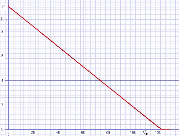
Now I_MAX and |Z_LIM| can be carried to the improved component calculation sequence above to finish the design.  The program of figure 14 below does just that.

Figure 14:  C++ code for calculation of safe-area limiter component values from power and current limit specifications.

/*     sal3.cpp - prove the equations calculated to define     a single-slope safe area limiter. */ #include <iostream> #include <cmath> using namespace std; #define PAR(x,y) ((x)*(y)/((x)+(y))) int main(void) {     double zlim, pmax, kv, ki, vt;     double r1, r2, r3, rs;     double vmax, imax;          // input values     imax = 10.0;     pmax = 300.0;     r3 = 47;     rs = 0.1;     vt = 0.763;     // calculate limit line specifications     zlim = 4*pmax/(imax*imax);     // remaining limit line specifications are informational     //   and not necessary to finish calculations     kv = sqrt((vt*vt)/(4.0*zlim*pmax));     ki = vt/imax;     kv = ki/zlim;     vmax = vt/kv;          // calculate component values     r2 = zlim*r3/rs;     // calculate r1 at midpoint     //r1 = vt/(((0.5*vmax)-vt)/r2+(rs*(0.5*imax)-vt)/r3);     // calculate r1 at current endpoint     r1 = vt/((-vt)/r2+(rs*imax-vt)/r3);     // print results     cout << "R2 = " << r2 << ",\t" << "R3 = " << r3 << endl;     cout << "R1 = " << r1 << ",\t" << "RS = " << rs << endl;     cout << "VT = " << vt << ",\t" << "PMAX = " << pmax;     cout << ",\t" << "ZLIM = " << zlim << endl;     cout << "Endpoints: " << vmax << "V,\t" << imax << "A" << endl;     return 0; }

Figure 15:  Program output for parameters given

R2 = 5640,    R3 = 47 R1 = 155.484,    RS = 0.1 VT = 0.763,    PMAX = 300,    ZLIM = 12 Endpoints: 120V,    10A

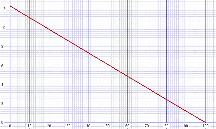
Figure 16:  SPICE plot of resulting load line

SPICE model

Compensation

Since the safe-area limiter is a feedback circuit under limit, a stability analysis might be in order to determine if a compensation capacitor is needed between the collector and base of Q₁.  A well-known designer always uses a 0.1µF capacitor in that location.

Not finished yet?

It remains to apply a safe-area limiter to a useful amplifier.

Document History
March 16, 2013  Created.
April 5, 2013  Added an improved component calculation sequence and additional power calculations.
December 9, 2015  Corrected two misspellings.